Case 3.2: KCS Deep water, trajectories
CASE 3.2: KCS in deep water
1. Description of case 3.2
- KCS hull shape, at even keel draught of 10.8 meter (full scale), model scale draught 0.285m.
- No bilge keels.
- Free to move in all directions.
- Starting speed: Fn = 0.26 (corresponding to full scale 24 knots).
- Calm water
- LPP = 6.0702 m (scale 37.89)
- g = 9.81 [m/s2], ρ=1000 [kg/m3]; ν=1.27×10⁻⁶ [m2/s]
- Propeller present and working at constant RPM. The RPM of the propeller is such that the ship is in (longitudinal) equilibrium at a speed of 24 knots full scale.
- Rudder (mariner type) steerable. The rudder rate will correspond to 2.32°/s on full scale or 14.28°/s on model scale
- GM is set to 0.6 meter (full scale), model scale value of 0.015835)
- Water depth is deep water, Wd/T = 17.5
- Radius of gyration for yaw and pitch are 0.258LPP (in air)
- Radius of gyration for roll is 0.4B (in air)
Case 3.2 consists of 5 cases: case 3.2.1 through 3.2.5, as explained below:
2. Experimental data
The submissions will be compared to model tests carried out by MARIN. Furthermore, there are 2 other sets of measurements, one set of IHI and one set of IIHR. They will help to obtain insight in the measurement uncertainty.
Further information: The roll decay result can be downloaded at
http://simman2019.kr/contents/KCS.php
3. Requested computations
The requested info comes in 5 pieces of information. In this way, we assure that at least for the 20°/20° zigzag test to portside, we have as many submissions as possible.
- You can only deliver case 3.2.2 when you deliver case 3.2.1.
- You can only deliver case 3.2.3 when you deliver case 3.2.2.
- You can only deliver case 3.2.4 when you deliver case 3.2.3.
- And so on
Table1: Requested information
| Package |
Manoeuvre |
Starting speed V0 |
| Case 3.2.1 |
Self propulsion information |
Fn = 0.26 (equivalent to 24 knots full scale) |
| Case 3.2.2 |
20°/20° zigzag test, starting to portside |
Fn = 0.26 (equivalent to 24 knots full scale) |
| Case 3.2.3 |
10°/10° zigzag test, starting to portside |
Fn = 0.26 (equivalent to 24 knots full scale) |
| Case 3.2.4 |
35° turning circle test, starting to portside |
Fn = 0.26 (equivalent to 24 knots full scale) |
| Case 3.2.5 |
20°/20° zigzag test, starting to starboard side |
Fn = 0.26 (equivalent to 24 knots full scale) |
The propeller RPM at t=0 should be such that the ship is in longitudinal equilibrium. So, for a CFD time domain simulations, the situation at t=0 is equivalent to a propulsion test! The analysers will look at this data.
3.1 Submission 3.2.1: Self-propulsion information
This submission is especially interesting for simulations based on URANS CFD. This case shows the “neutral rudder angle”, and the obtained longitudinal equilibrium (the propeller rpm and thrust). For simulations based on coefficient models, the neutral angle will often be zero.
- All results are to be given for model scale conditions.
- All simulations results should be provided in the format described in section 4.
- The propeller rate of revolution should correspond to the self-propulsion point of the model. When the RPM is unknown (because for example a constant thrust or actuator disk model is used in CFD based simulations) please indicate this.
- Similar to the experiment, the rudders should be controlled by following autopilot during course keeping:
where δ(t) is rudder angle, proportional gain KP is 1.0, KD is 18.5 on full scale, 3 on model scale. ψC is the target yaw angle and ψ(t) is yaw angle. The maximum rudder rate should be assigned to 14.28 [deg/s], model scale. Rudder angle should be controlled by P controller during approaching before starting rudder execution for manoeuvring (Target yaw angle: ψC=0°)
Please see section 5 for an example of the submission.
3.2 Submission 3.2.2: 20°/20° zigzag manoeuvre starting to portside
- All results are to be given for model scale conditions.
- All simulations results should be provided in the format described in section 4.
- The propeller rate of revolution should correspond to the self-propulsion point of the model. When the RPM is unknown (because for example a constant thrust or actuator disk model is used in CFD based simulations) please indicate this.
- Similar to the experiment, the rudders are controlled by autopilot during approaching before starting rudder execution for starboard side zigzag.
- During the zigzag maneuver, the rudders should go to the real geometric 20 degrees (not to 20 degrees away from the neutral angle).
- The heading at which the rudder goes to the opposite side is 20 degrees.
Please see section 6 for an example of the submission.
3.3 Submission 3.2.3: 10°/10° zigzag manoeuvre starting to portside
- All results are to be given for model scale conditions.
- All simulations results should be provided in the format described in section 4.
- The propeller rate of revolution should correspond to the self-propulsion point of the model. When the RPM is unknown (because for example a constant thrust or actuator disk model is used in CFD based simulations) please indicate this.
- Similar to the experiment, the rudders are controlled by autopilot during approaching before starting rudder execution for starboard side zigzag.
- During the zigzag maneuver, the rudders should go to the real geometric 10 degrees (not to 10 degrees away from the neutral angle).
- The heading at which the rudder goes to the opposite side is 10 degrees.
Please see section 7 for an example of the submission.
3.4. Submission 3.2.4: 35° portside turning circle maneuver
- All results are to be given for model scale conditions.
- All simulations results should be provided in the format described in section 4.
- The propeller rate of revolution should correspond to the self-propulsion point of the model. When the RPM is unknown (because for example a constant thrust or actuator disk model is used in CFD based simulations) please indicate this.
- Similar to the experiment, the rudders are controlled by autopilot during approaching before starting rudder execution for starboard side zigzag.
- During the zigzag maneuver, the rudders should go to the real geometric 35 degrees (not to 35 degrees away from the neutral angle).
Please see section 8 for an example of the submission.
3.5. Submission 3.2.5: 20°/20° zigzag manoeuvre starting to starboard
- All results are to be given for model scale conditions.
- All simulations results should be provided in the format described in section 4.
- The propeller rate of revolution should correspond to the self-propulsion point of the model. When the RPM is unknown (because for example a constant thrust or actuator disk model is used in CFD based simulations) please indicate this.
- Similar to the experiment, the rudders are controlled by autopilot during approaching before starting rudder execution for starboard side zigzag.
- During the zigzag maneuver, the rudders should go to the real geometric 20 degrees (not to 20 degrees away from the neutral angle).
- The heading at which the rudder goes to the opposite side is 20 degrees.
Please see section 9 for an example of the submission.
4. Format
Time series of the manoeuvres should be send to the organizers in an excel file. The data shall be give on model scale, and it will be compared to model scale data.
The submission consists of an excel file (example is given) with 17 columns and with rows for every time step. The time step is free to chose, but a small enough time step somewhere around 0.05 to 0.01 is recommended to get sufficient accuracy. The following quantities are asked:
Table 2: Submission variables
| Symbol |
Item |
Unit |
| t |
time |
s |
| X |
X position in earth fixed system |
m |
| Y |
Y position in earth fixed system |
m |
| z |
z position in earth fixed system |
m |
| ϕ |
Roll angle |
degrees |
| θ |
Pitch angle |
degrees |
| ψ |
Yaw angle |
degree |
| u |
surge velocity in horizontal-body-fixed coordinate system |
m/s |
| v |
sway velocity in horizontal-body-fixed coordinate system |
m/s |
| w |
heave velocity |
m/s |
| p |
roll rate |
deg/s |
| q |
pitch rate |
deg/s |
| r |
yaw rate in body-fixed coordinate system |
deg/s |
| δ |
Rudder angle |
deg |
| n |
Propeller revolutions/td>
| rpm |
| T |
Thrust of propeller |
N |
| Q |
Torque of propeller |
Nm |
| FR |
Rudder normal force (except horn part) |
N |
These data are illustrated in Figure 1. The origin is located on O. The time t=0 is the time when the steering starts. The initial direction of the model is the direction of X-axis. Initial conditions at t = 0 are: X
0=0, Y
0=0, u=U
0, r=0, δ=δ
0 (which is the neutral rudder angle)
 Figure 1: Illustration of the sign convention of the earth-fixed and body-fixed coordinate system.
Notes:
- The ship position or trajectory should be given in an Earth-fixed coordinate system with X pointing North, Y pointing East, and Z pointing downward as shown in Figure 1. This x0y0z0 axis system remains horizontal in the earth. The ship was released at (0,0) when t = 0 . The roll angle (ϕ) is positive for pushing starboard into the water, pitch (θ) is positive for bow up position and yaw angle (ψ) is positive for bow turned to starboard. The reported trajectory is dimensional and angular motions should be reported in degrees. The angular velocities should be reported in degree per second. The reported yaw angle should be the deviation of yaw angle respect to the target yaw i.e. ψ-ψC.
- All velocities for 6DOF motions (u, v, w p, q r) should be reported in ship-fixed coordinate system with x axis positive toward bow, y axis positive toward starboard and z axis positive downward. This xyz axis system rotates with the ship in yaw but not pitch and roll, i.e., remains horizontal in the earth. It is a so-called “yawed-only reference system”. Given this convention, the reported velocities are:
 (3)
(3)
 (4)
(4)
In Equation (4), the unit of p, r,  , and
, and  is [deg/s]. Rudder angle (δ) is positive when trailing edge moves to portside.
- The thrust T and torque Q for each propeller should be reported in shaft coordinate system with x axis positive toward the engine. Values are given dimensional
- All motions should be reported at O.
- Link to an excel file case 3.2.1, in which the submitter can put his data.
- Link to an excel file case 3.2.2, in which the submitter can put his data.
- Link to an excel file case 3.2.3, in which the submitter can put his data.
- Link to an excel file case 3.2.4, in which the submitter can put his data.
- Link to an excel file case 3.2.5, in which the submitter can put his data.
- Link to an excel file, in which the submitter can put the details of the calculation method.
The yellow fields in the excel sheet should be filled in. The excel sheet should be send to the organizing committee per email address “
simman2019host@gmail.com”.
5. Elaborated example of case 3.2.1 (self propulsion data)
For case 3.2.1, we will ask the equilibrium speeds u, v, the rudder angle, RPM (i.e. the neutral rudder angle), thrust and torque, when available in the used method.
6. Elaborated example of case 3.2.2 (20/20 zigzag test, starting to portside)
For case 3.2.2, the comparison will look as displayed in the following figure 2. As can be seen, the results of the time traces will be analysed and presented non-dimensional. On top of the time traces as presented in figure 2, the values of overshoot angles, rates of turn, period, etc will be derived from the time series. Table 2 illustrated which characteristics will be derived from the time series. These characteristics will be compared too as displayed in the figure 3: this shows how three submissions are compared to the FRMT data. A statistical analysis will be performed for all submissions to observe the spreading in results.
The primary values for the comparison will be the 1
st and 2
nd overshoot angles.
The secondary values for the comparison will be the period, the rate of turn during 1
st and 2
nd oscillation.
Table 3: Comparison values for Case 2.2.2
| Category |
Unit |
Validation Variables |
| Overshoot angles |
[deg] |
1st overshoot angle (ψOS1) |
|
[deg] |
2nd overshoot angle (ψOS2) |
|
[deg] |
3nd overshoot angle (ψOS3) |
| Time of execute |
[s] |
Time of 2nd rudder execute (t2) |
|
[s] |
Time of 3rd rudder execute (t3) |
|
[s] |
Time of 4th rudder execute (t4) |
| Times |
[s] |
Period (time between the 4th and 2nd rudder execute = t4-t2) |
|
[s] |
1st overshoot time (tOS1) |
|
[s] |
2nd overshoot time (tOS2) |
|
[s] |
3rd overshoot time (tOS3) |
| Maximum yaw rate |
[deg/s] |
Maximum yaw rate during 1st overshoot between t2 and t3 (r1) |
|
[deg/s] |
Maximum yaw rate during 2nd overshoot between t3 and t4 (r2) |
|
[deg/s] |
Maximum yaw rate during 3rd overshoot between t4 and t5 (r3) |
| Maximum drift angle |
[deg] |
Maximum drift angle during 1st overshoot between t2 and t3 (β1) |
|
[deg] |
Maximum drift angle during 2nd overshoot between t3 and t4 (β2) |
|
[deg] |
Maximum drift angle during 3rd overshoot between t4 and t5 (β3) |
| Maximum roll angle |
[deg] |
Maximum roll angle during 1st overshoot between t2 and t3 (ϕ1) |
|
[deg] |
Maximum roll angle during 2nd overshoot between t3 and t4 (ϕ2) |
|
[deg] |
Maximum roll angle during 3rd overshoot between t4 and t5 (ϕ3) |
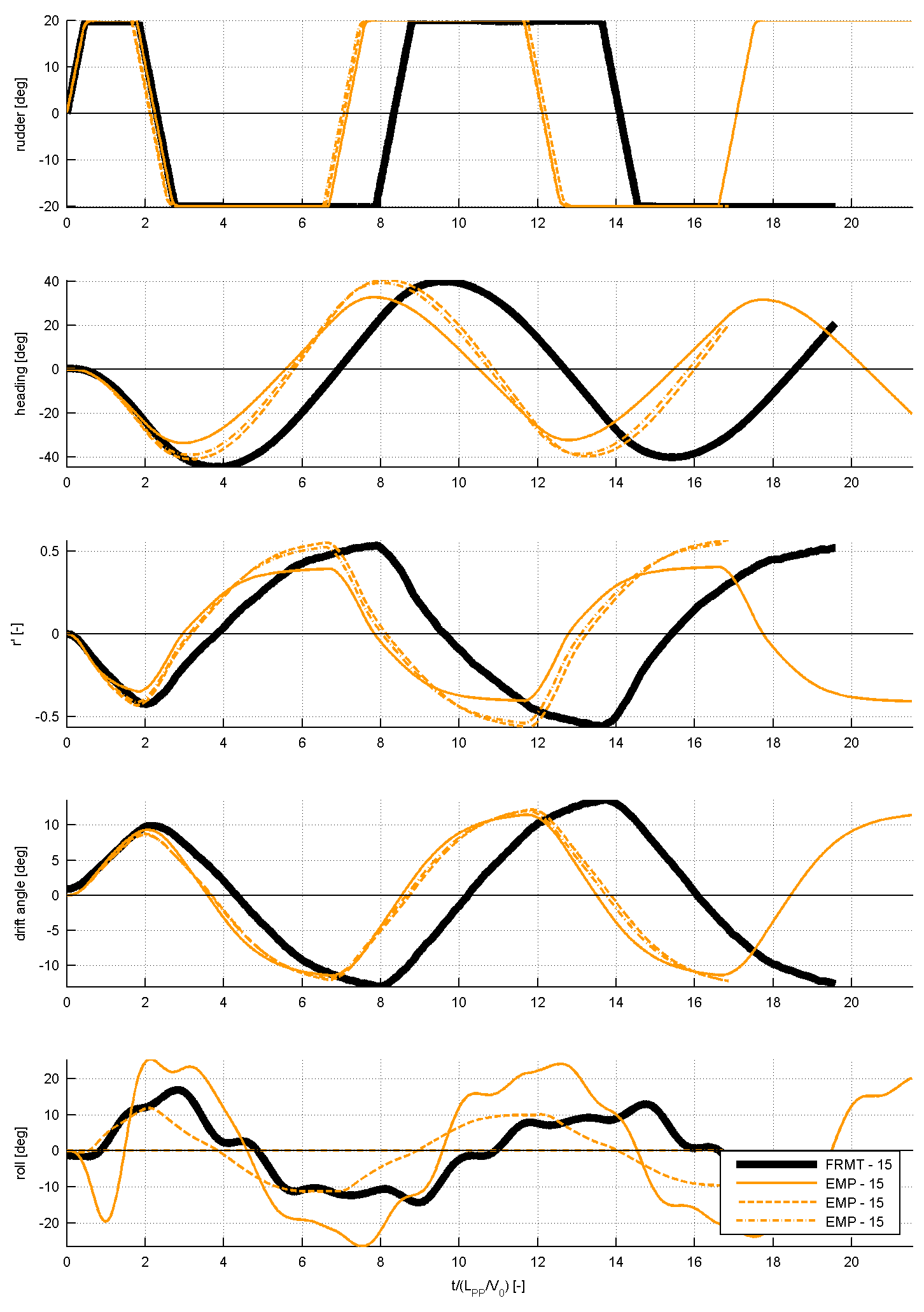 Figure 2: time traces of several submissions for the 20/20 zig-zag manoeuvre, compared to FRMT
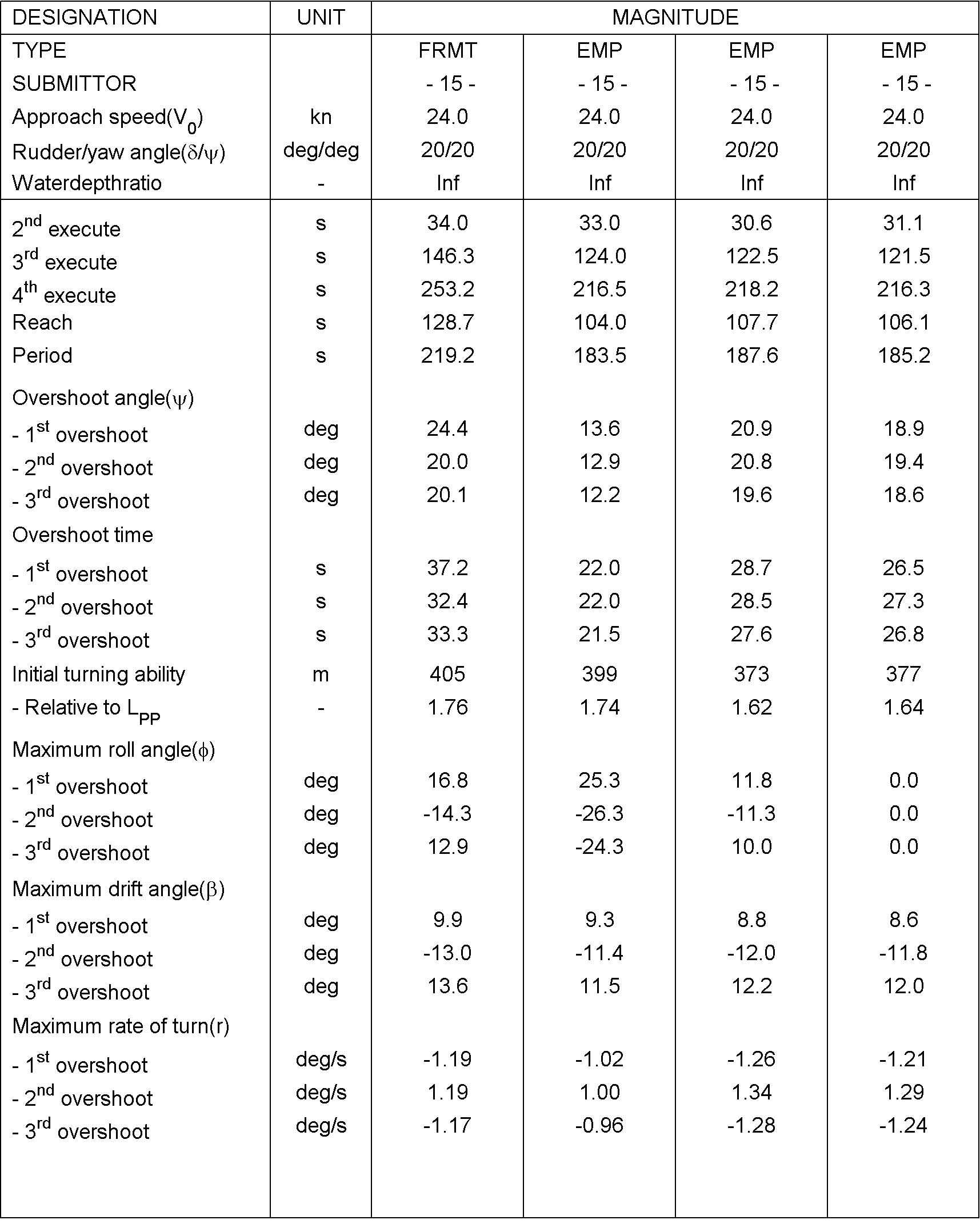 Figure 3: derived characteristics for the 20/20 zigzag manoeuvre to portside
7. Elaborated example of case 3.2.3 (10/10 zigzag test, starting to portside)
For case 3.2.3, the comparison will look as displayed in the following figure 4. As can be seen, the results of the time traces will be analysed and presented non-dimensional. On top of the time traces as presented in figure 4, the values of overshoot angles, rates of turn, period, etc will be derived from the time series. Table 3 illustrated which characteristics will be derived from the time series. These characteristics will be compared too as displayed in the figure 5: this shows how three submissions are compared to the FRMT data. A statistical analysis will be performed for all submissions to observe the spreading in results.
The primary values for the comparison will be the 1
st and 2
nd overshoot angles and the initial turning ability.
The secondary values for the comparison will be the period, the rate of turn during 1
st and 2
nd oscillation.
Table 4: Comparison values for Case 3.2.3
| Category |
Unit |
Validation Variables |
| Overshoot angles |
[deg] |
1st overshoot angle (ψOS1) |
|
[deg] |
2nd overshoot angle (ψOS2) |
|
[deg] |
3nd overshoot angle (ψOS3) |
| Initial turning ability |
[LPP] |
Initial turning ability ITA |
| Time of execute |
[s] |
Time of 2nd rudder execute (t2) |
|
[s] |
Time of 3rd rudder execute (t3) |
|
[s] |
Time of 4th rudder execute (t4) |
| Times |
[s] |
Period (time between the 4th and 2nd rudder execute = t4-t2) |
|
[s] |
1st overshoot time (tOS1) |
|
[s] |
2nd overshoot time (tOS2) |
|
[s] |
3rd overshoot time (tOS3) |
| Maximum yaw rate |
[deg/s] |
Maximum yaw rate during 1st overshoot between t2 and t3 (r1) |
|
[deg/s] |
Maximum yaw rate during 2nd overshoot between t3 and t4 (r2) |
|
[deg/s] |
Maximum yaw rate during 3rd overshoot between t4 and t5 (r3) |
| Maximum drift angle |
[deg] |
Maximum drift angle during 1st overshoot between t2 and t3 (β1) |
|
[deg] |
Maximum drift angle during 2nd overshoot between t3 and t4 (β2) |
|
[deg] |
Maximum drift angle during 3rd overshoot between t4 and t5 (β3) |
| Maximum roll angle |
[deg] |
Maximum roll angle during 1st overshoot between t2 and t3 (ϕ1) |
|
[deg] |
Maximum roll angle during 2nd overshoot between t3 and t4 (ϕ2) |
|
[deg] |
Maximum roll angle during 3rd overshoot between t4 and t5 (ϕ3) |
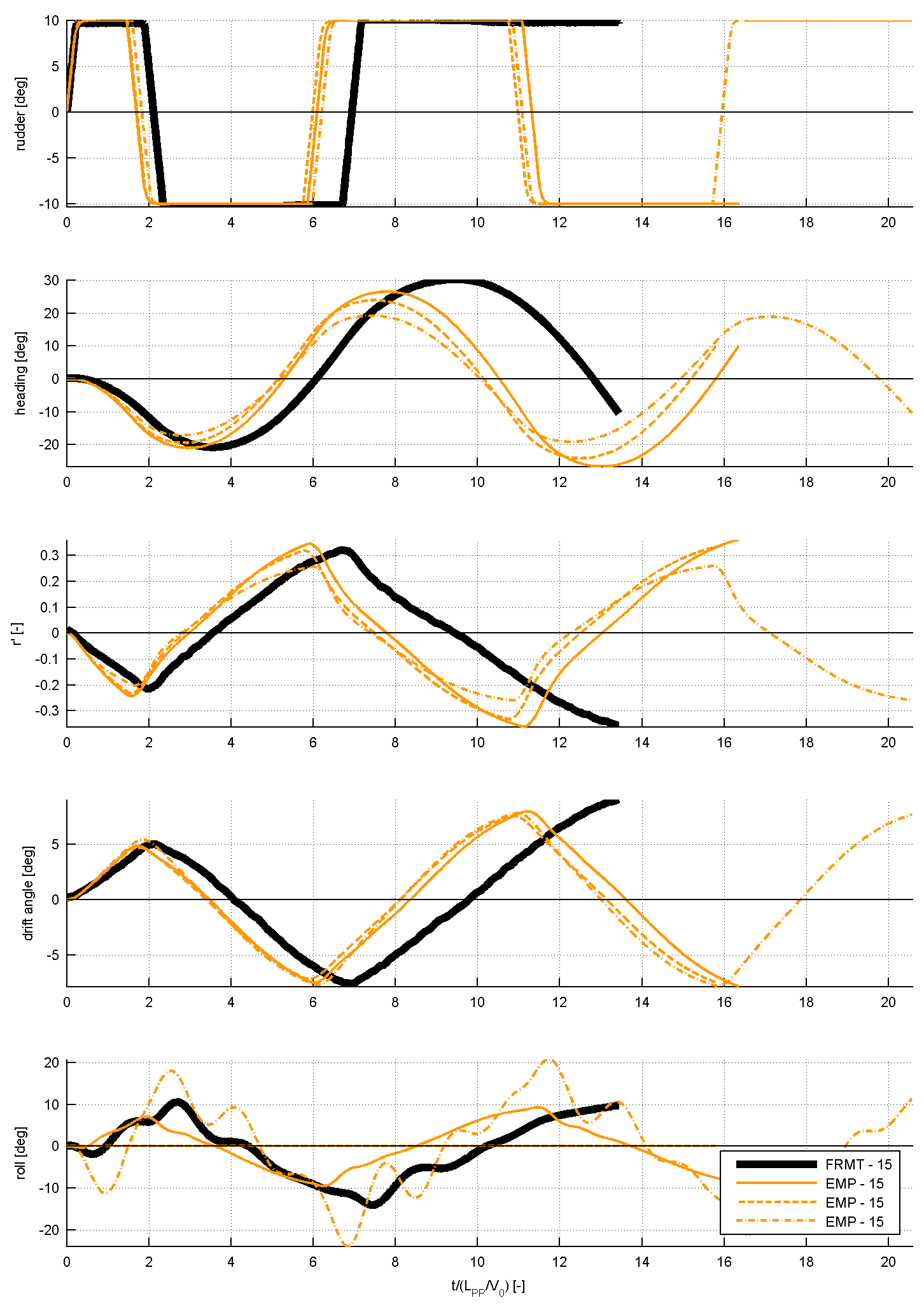 Figure 4: time traces of several submissions for the 10/10 zig-zag manoeuvre, compared to FRMT
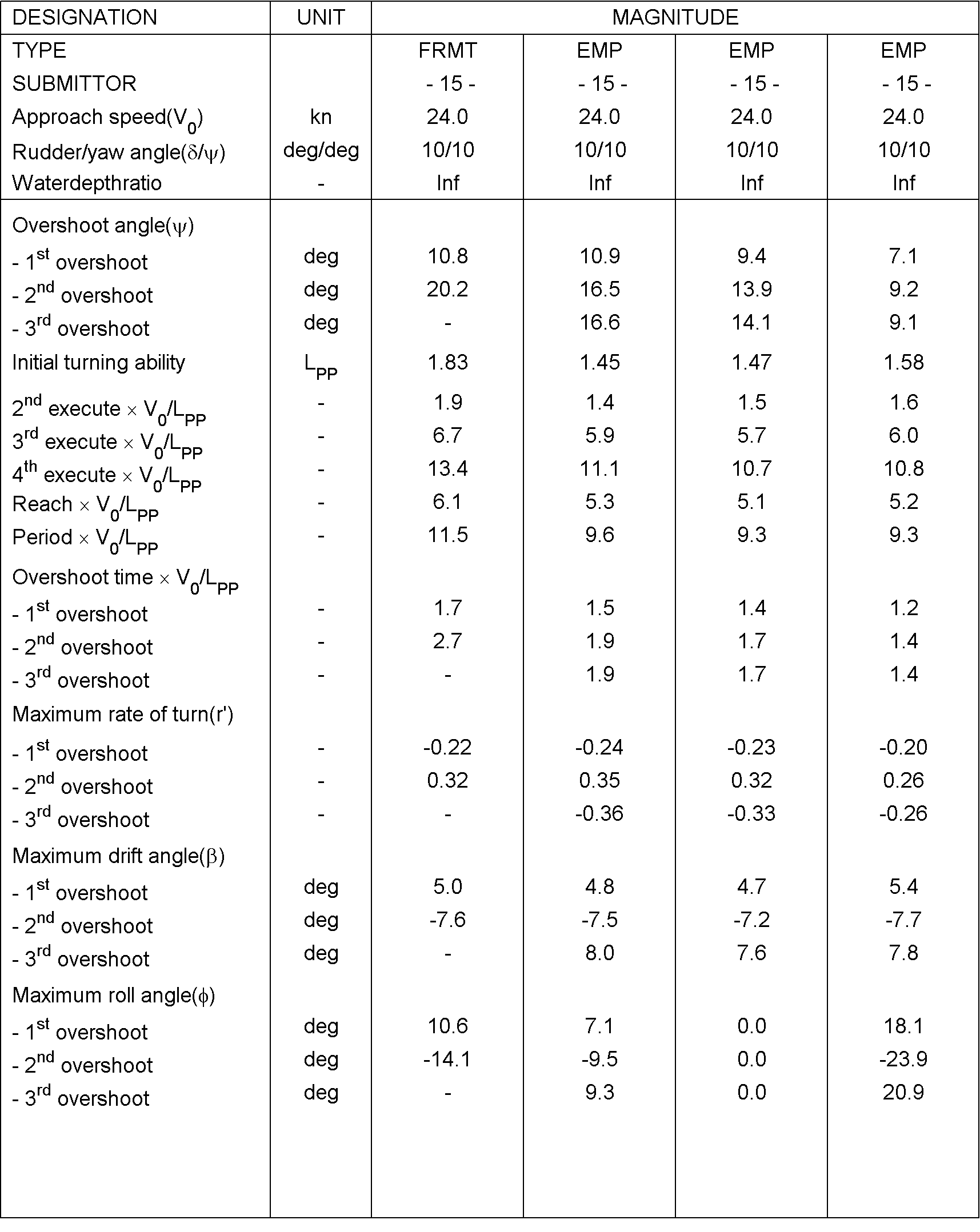 Figure 5: derived characteristics for the 10/10 zigzag manoeuvre to portside
8. Elaborated example of case 3.2.4 (35° turning circle manoeuvre, starting to portside)
For case 3.2.4, the comparison will look as displayed in the following figure 6 and 7. As can be seen, the results of the time traces will be analysed and presented non-dimensional. On top of the time traces as presented in figure 4, the values of tactical diameter, rate of turn, drift angle, speed loss, etc will be derived from the time series. Table 3 illustrated which characteristics will be derived from the time series. These characteristics will be compared too as displayed in the figure 5: this shows how three submissions are compared to the FRMT data. A statistical analysis will be performed for all submissions to observe the spreading in results.
The primary values for the comparison will be the advance and tactical diameter. The secondary values for the comparison are indicated in the table 4.
Table 5: Comparison values for Case 3.2.4
| Category |
Unit |
Validation Variables |
| Dimensions |
[-] |
Advance / LPP (Ad/LPP) |
|
[-] |
Tactical diameter / LPP (TD/LPP) |
|
[-] |
Transfer / LPP (Tr/LPP) |
| Times |
[s] |
Time to reach 90° (t90°) |
|
[s] |
Time to reach 180° (t180°) |
|
[s] |
Time to reach 36° (t360°) |
| Yaw rate |
[deg/s] |
Maximum yaw rate (rmax) |
|
[deg/s] |
Average yaw rate in the constant part of the turn (rC) |
| Speed |
[m/s] |
Speed in the steady part of the turn (UC) |
| Roll |
[deg] |
Maximum inward roll angle (ϕinmax) |
|
[deg] |
Maximum outward roll angle (ϕoutmax) |
|
[deg] |
Roll angle in the constant part of the turn (ϕc) |
| Non-dimensional values |
[-] |
Non-dimensional yaw rate in the constant part of the turn (r’) |
|
[deg] |
Drift angle in the constant part of the turn (βC) |
|
[-] |
Pivot point (-sin(βC)/r’) |
|
[-] |
Speed ratio (UC/U0) |
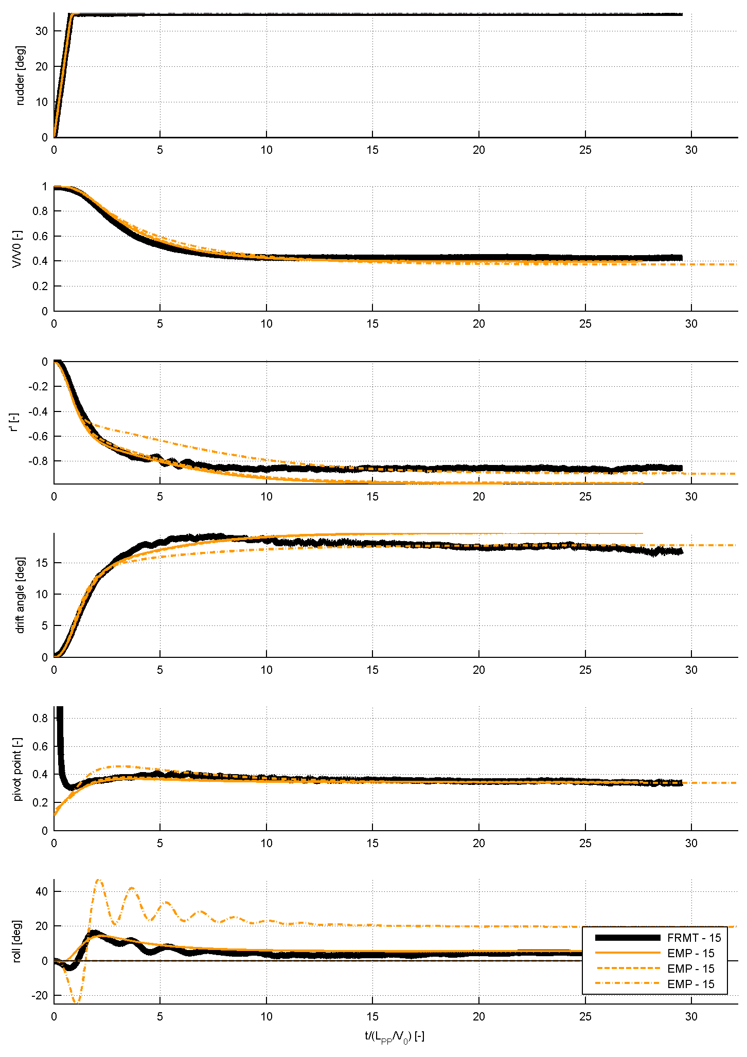 Figure 6: time traces of several submissions for the 35 degrees turning circle manoeuvre, compared to FRMT
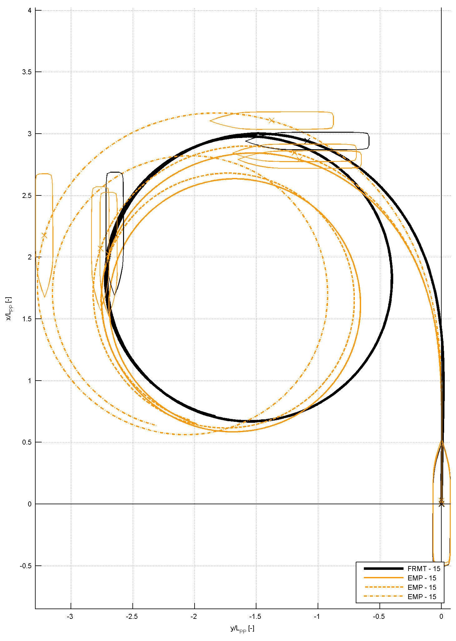 Figure 7: time traces of several submissions for the 10/10 zig-zag manoeuvre, compared to FRMT
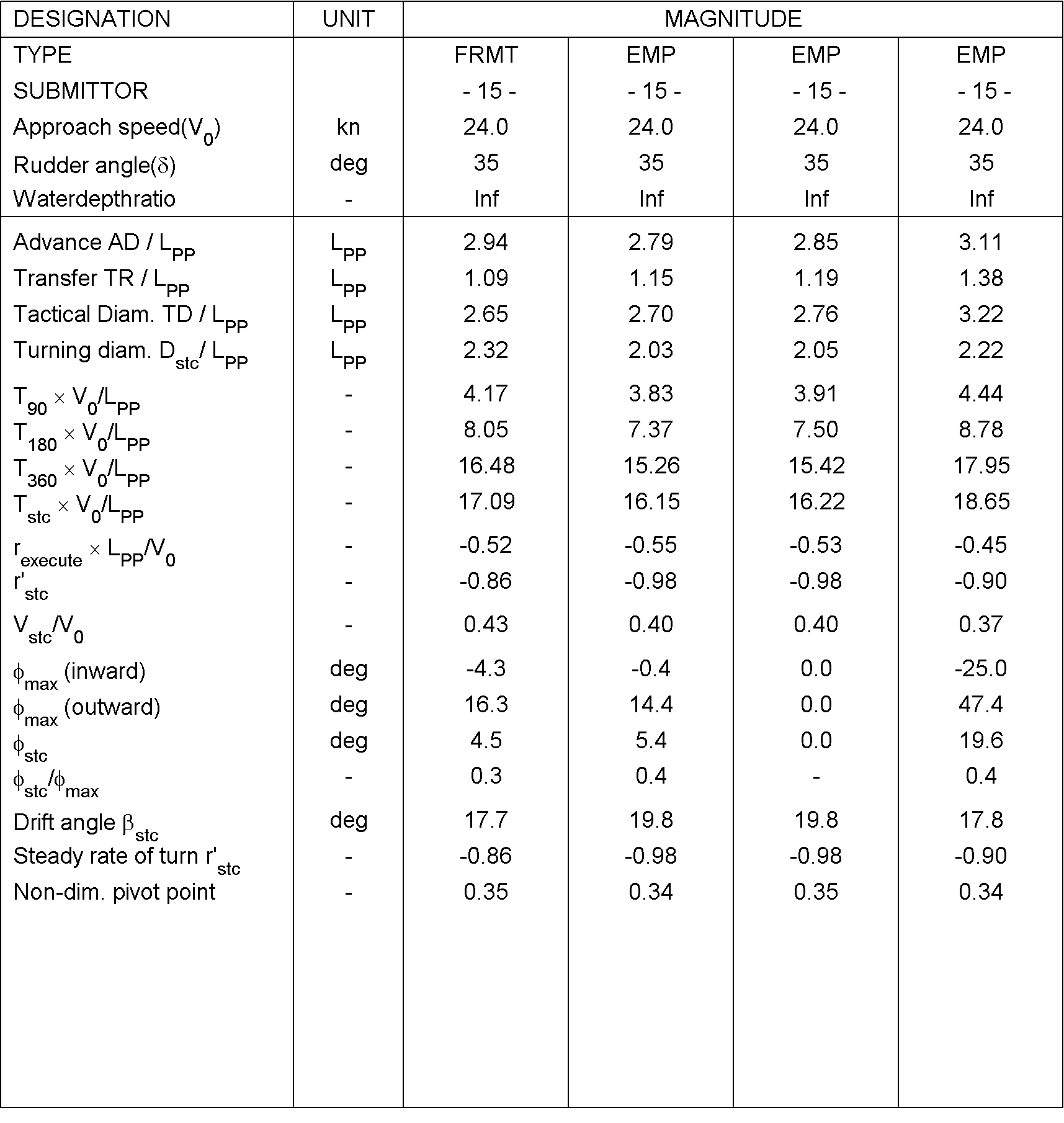 Figure 8: derived characteristics for the 35 degrees turning circle manoeuvre to portside
9. Elaborated example of case 3.2.5 (20/20 zigzag test, starting to starboard side)
For case 3.2.5, the comparison will look as displayed in the following figure 9. As can be seen, the results of the time traces will be analysed and presented non-dimensional. On top of the time traces as presented in figure 9, the values of overshoot angles, rates of turn, period, etc will be derived from the time series. Table 6 illustrated which characteristics will be derived from the time series. These characteristics will be compared too as displayed in the figure 10: this shows how three submissions are compared to the FRMT data. A statistical analysis will be performed for all submissions to observe the spreading in results.
The primary values for the comparison will be the 1
st and 2
nd overshoot angles.
The secondary values for the comparison will be the period, the rate of turn during 1
st and 2
nd oscillation.
Table 6: Comparison values for Case 3.2.5
| Category |
Unit |
Validation Variables |
| Overshoot angles |
[deg] |
1st overshoot angle (ψOS1) |
|
[deg] |
2nd overshoot angle (ψOS2) |
|
[deg] |
3nd overshoot angle (ψOS3) |
| Time of execute |
[s] |
Time of 2nd rudder execute (t2) |
|
[s] |
Time of 3rd rudder execute (t3) |
|
[s] |
Time of 4th rudder execute (t4) |
| Times |
[s] |
Period (time between the 4th and 2nd rudder execute = t4-t2) |
|
[s] |
1st overshoot time (tOS1) |
|
[s] |
2nd overshoot time (tOS2) |
|
[s] |
3rd overshoot time (tOS3) |
| Maximum yaw rate |
[deg/s] |
Maximum yaw rate during 1st overshoot between t2 and t3 (r1) |
|
[deg/s] |
Maximum yaw rate during 2nd overshoot between t3 and t4 (r2) |
|
[deg/s] |
Maximum yaw rate during 3rd overshoot between t4 and t5 (r3) |
| Maximum drift angle |
[deg] |
Maximum drift angle during 1st overshoot between t2 and t3 (β1) |
|
[deg] |
Maximum drift angle during 2nd overshoot between t3 and t4 (β2) |
|
[deg] |
Maximum drift angle during 3rd overshoot between t4 and t5 (β3) |
| Maximum roll angle |
[deg] |
Maximum roll angle during 1st overshoot between t2 and t3 (ϕ1) |
|
[deg] |
Maximum roll angle during 2nd overshoot between t3 and t4 (ϕ2) |
|
[deg] |
Maximum roll angle during 3rd overshoot between t4 and t5 (ϕ3) |
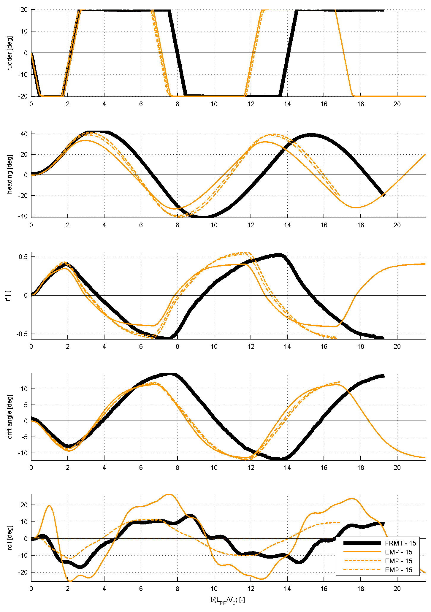 Figure 9: time traces of several submissions for the 20/20 zig-zag manoeuvre to starboard, compared to FRMT
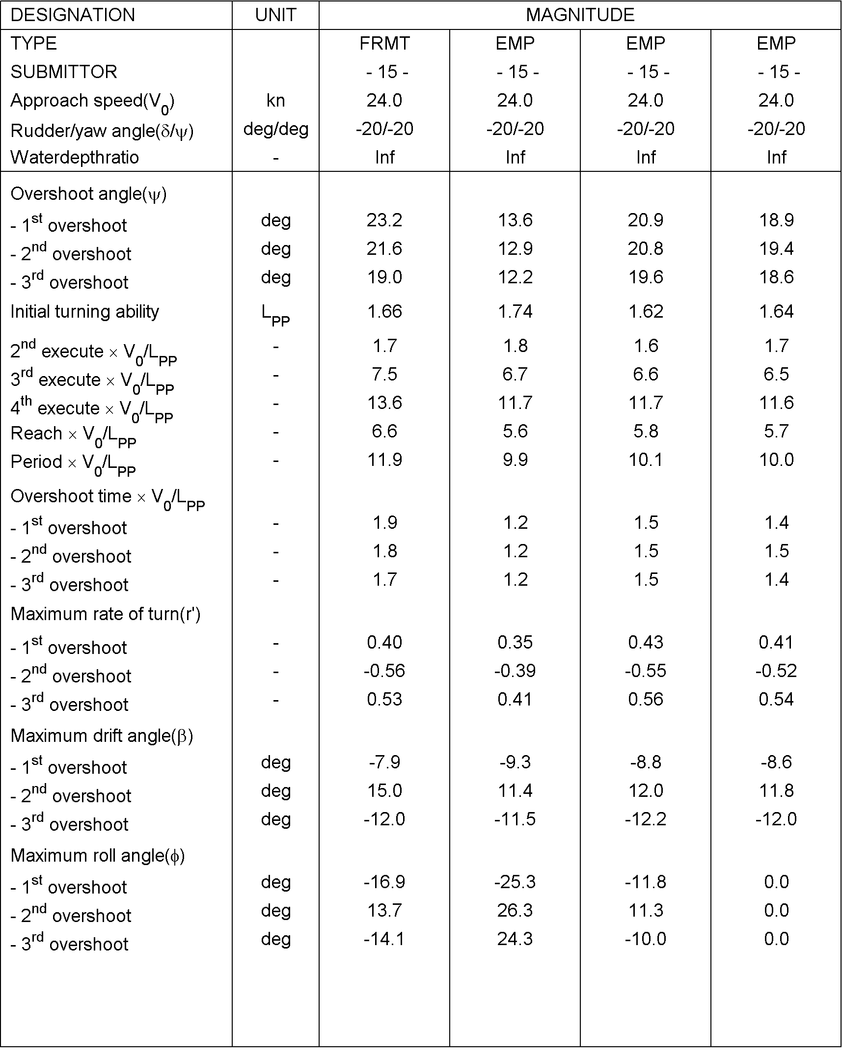 Figure 10: derived characteristics for the 20/20 zigzag manoeuvre to starboard side